Example Analysis

Dataset

The dataset is taken from Mahler et al. (2013)¹. It is embedded in the package, so that we can load it and plot it using ape base functions.

library(cauphy)
data(lizards)
attach(lizards)

plot(phy, show.tip.label = FALSE, x.lim = 65)
phydataplot(svl, phy, scaling = 2)
nodelabels(node = c(142, 151, 157))

The phylogeny is a time calibrated tree, and the trait is the natural log-transformed species average snout-to-vent length (in centimeters) of lizard species.

Cauchy Process Fit - REML

The fitCauchy function can fit a Cauchy process (CP) to the data, using the REML by default.

cauchy_reml <- fitCauchy(phy, svl, model = "cauchy", method = "reml")
cauchy_reml
#> Call:
#> fitCauchy(phy = phy, trait = svl, model = "cauchy", method = "reml")
#> 
#>                 AIC logLik (restricted) 
#>              -4.207               3.104 
#> 
#> Parameter estimate(s) using REML:
#> dispersion: 0.004476062

The print method shows the main information of the plot, including the (restricted) likelihood and AIC values, and the parameter estimates.

Estimated confidence intervals for the parameters can be obtained through the numerical computation of the Hessian.

confint(cauchy_reml)
#> Approximated asymptotic confidence interval using the Hessian.
#>            2.5 %      97.5 %
#> disp 0.003178267 0.005773856

We can also plot the profile likelihood around the inferred parameter value, in order to check that the numerical optimization went well, and that the likelihood computation did not encounter some numerical robustness issues.

prl <- profile(cauchy_reml)
plot(prl)

Here, the likelihood is smooth, and has a clear maximum in the estimated dispersion value.

Cauchy Process Fit - ML

It is also possible to directly fit the maximum likelihood, instead of the REML, in this case with a fixed root.

cauchy_ml <- fitCauchy(phy, svl, model = "cauchy", method = "fixed.root")
cauchy_ml
#> Call:
#> fitCauchy(phy = phy, trait = svl, model = "cauchy", method = "fixed.root")
#> 
#>    AIC logLik 
#> -4.884  4.442 
#> 
#> Parameter estimate(s) using ML:
#> dispersion: 0.00450843 
#> root value: 3.9951

In this case, both the root value and the dispersion are estimated using ML, and their confidence interval can also be approximated using the Hessian.

confint(cauchy_ml)
#> Approximated asymptotic confidence interval using the Hessian.
#>            2.5 %      97.5 %
#> x0   3.787157040 4.203042999
#> disp 0.003207639 0.005809221

Note that in this case with many tips, the difference between the ML and REML estimates of the dispersion are small.

Finally, we can also plot the profile log-likelihood in both estimated parameters (the other parameter being fixed to its optimal value). Here again, the likelihood surface seems to be smooth and have a clear maximum.

prl <- profile(cauchy_ml)
plot(prl)

Model Selection

We can use either ML or REML for model selection, comparing the AIC value of the Cauchy fit with those of Gaussian models.

Here, we use phylolm to fit Gaussian models, which uses an ML estimate (with fixed root). We only compare the CP with the BM, OU and EB without measurement error for simplicity, but results for other Gaussian models are similar.

library(phylolm)
bm_ml <- phylolm(svl ~ 1, phy = phy, model = "BM")
ou_ml <- phylolm(svl ~ 1, phy = phy, model = "OUfixedRoot")
eb_ml <- phylolm(svl ~ 1, phy = phy, model = "EB")

data.frame(model = c("BM", "OU", "EB", "CP"),
           AIC = c(AIC(bm_ml), AIC(ou_ml), AIC(eb_ml), AIC(cauchy_ml)))
#>   model       AIC
#> 1    BM 13.400807
#> 2    OU 15.400810
#> 3    EB 14.571939
#> 4    CP -4.883842

Here, the Cauchy Process is clearly selected by the AIC score.

Ancestral Trait Reconstruction

For ancestral trait reconstruction, we compute the posterior trait density conditionally on the tip values, given a fitted object.

To do ancestral state reconstruction, we use the REML fitted object. The ML fitted object could also be used, and would give similar results, except for the root, which can be reconstructed in the REML case, but is fixed in the ML case.

anc_reml <- ancestral(cauchy_reml, n_values = 200)

We reconstruct the posterior density of each internal node on a grid of values. A default grid with $100$ is used if un-specified, but it can be tailored to specific needs by raising the number of points on the grid, or directly specifying a custom grid of values. By default, the reconstruction is carried on all internal nodes, but a subset of nodes of interest can be specified.

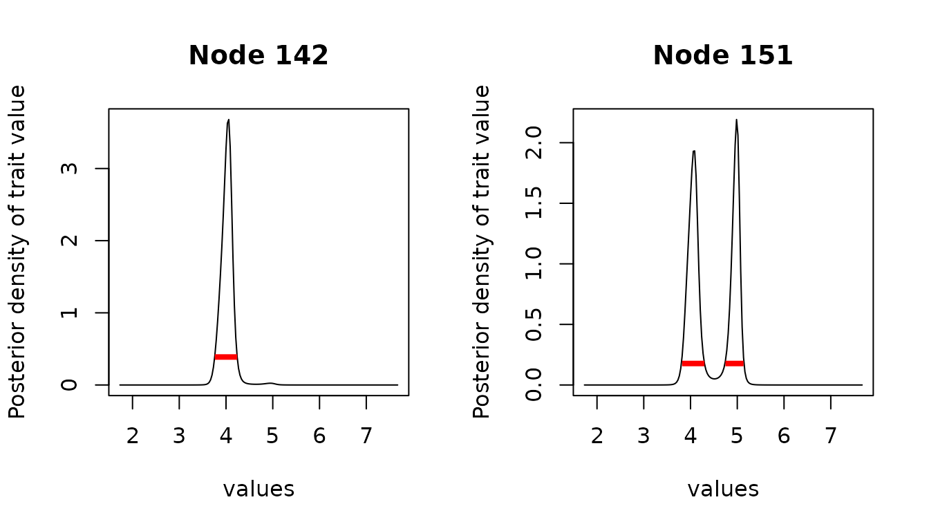
The posterior density can be plotted for specific nodes of interests. Here, node $151$ exhibits a bi-modal behavior, between “large” and “small” values of the trait at this internal node, representing two possible evolutionary scenarios.

plot(anc_reml, node = c(142, 151), type = "l")

Using the HDInterval package, it is possible to compute Highest (Posterior) Density Intervals for ancestral nodes, using the density estimated on the grid.

library(HDInterval)
anc_int <- hdi(anc_reml) # defaults to 95% HDI
plot(anc_reml, node = c(142, 151), intervals = anc_int, type = "l")

The hdi function can recover discontinuous intervals (thanks to the allowSplit option, see documentation), which can be relevant for multi-modal reconstructed densities, such as node 151 here.

anc_int[["151"]]
#>         begin      end
#> [1,] 3.820448 4.298035
#> [2,] 4.745773 5.133812
#> attr(,"credMass")
#> [1] 0.95
#> attr(,"height")
#> [1] 0.1772771

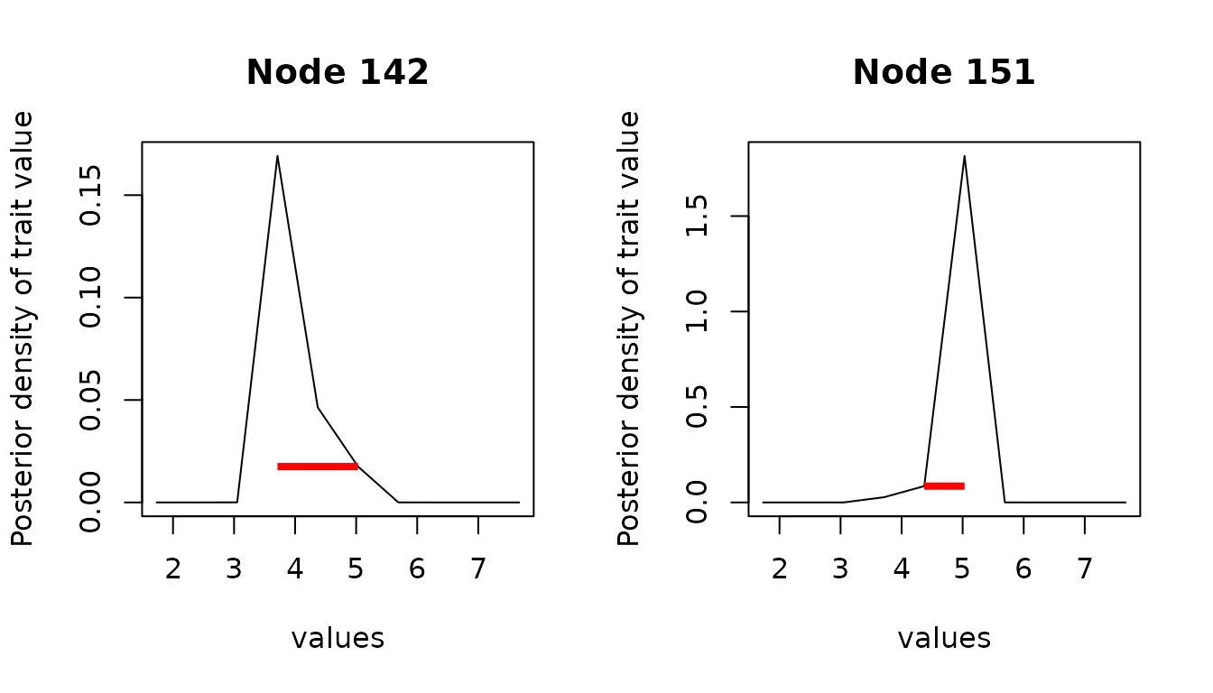
Note that the quality of the estimation of the interval depends on the quality of the estimation of the ancestral density. In particular, if the grid is inadequate or too coarse, then the resulting intervals can be meaningless.

anc_bad <- ancestral(cauchy_reml, n_values = 10) # grid is too coarse
anc_int_bad <- hdi(anc_bad)
plot(anc_bad, node = c(142, 151), intervals = anc_int_bad, type = "l")

Ancestral Branch Increment Reconstruction

Ancestral branch increment reconstruction computes the posterior density of the increment of a trait on each branch of the tree. Large branch increments can be associated with shifts on the trait value.

The process is similar to ancestral reconstruction, but is computationally more expensive. A built-in option can allow for parallelization of these computations. To avoid long run times, we only reconstruct the increment on a few chosen branches here.

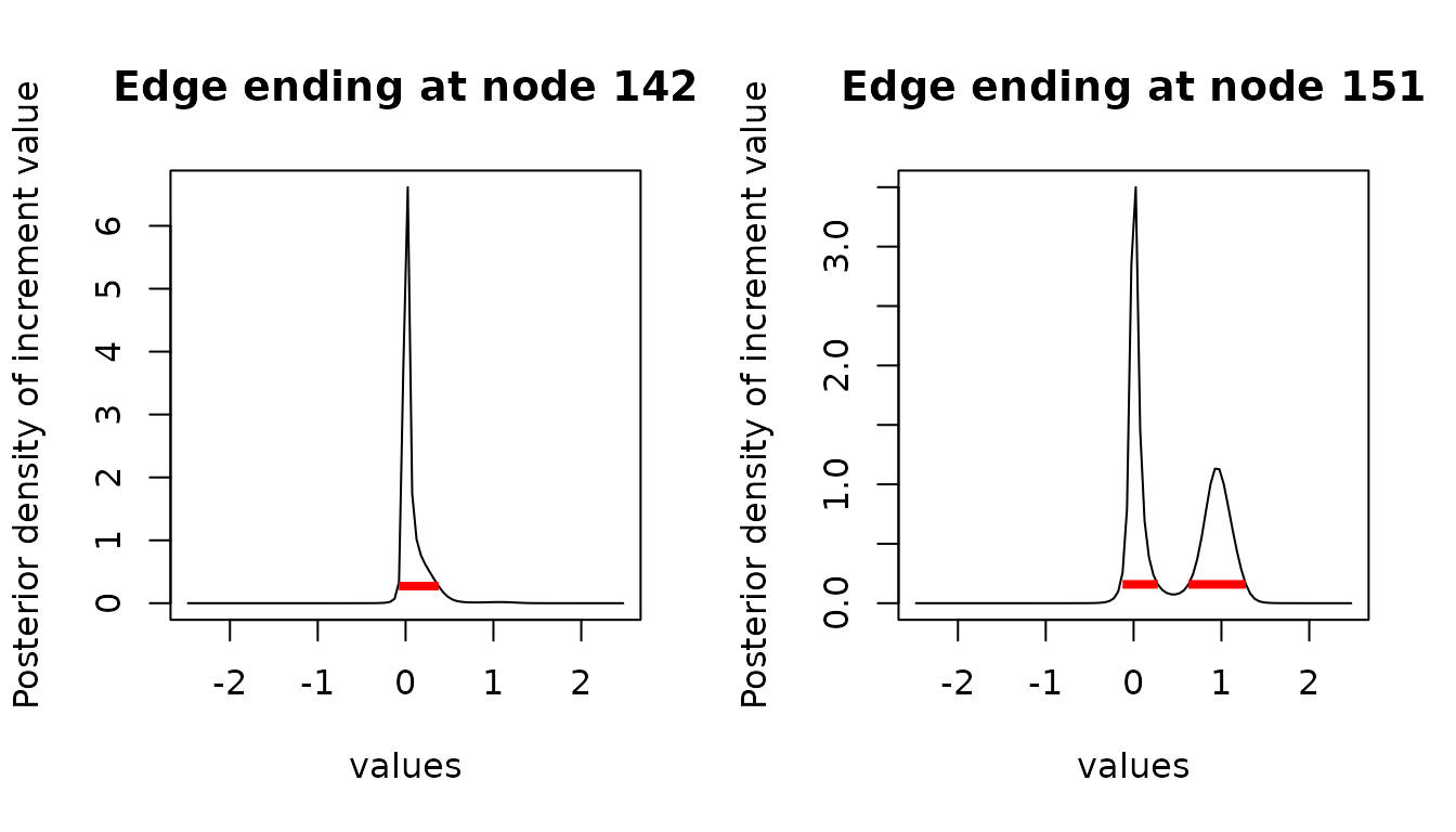
inc_reml <- increment(cauchy_reml, node = c(142, 151, 157), n_cores = 1)

We recover here a behavior that is complementary to the node reconstruction, with the edge ending at node $151$ being bi-modal, with modes around $0$ (no change on the edge) and $1$ (shift in the log trait space).

plot(inc_reml, node = c(142, 151), type = "l")

We can again compute and plot the HDI for the ancestral increments:

inc_int <- hdi(inc_reml) # defaults to 95% HDI
plot(inc_reml, node = c(142, 151), intervals = inc_int, type = "l")

Schematic Plot of Ancestral Reconstructions

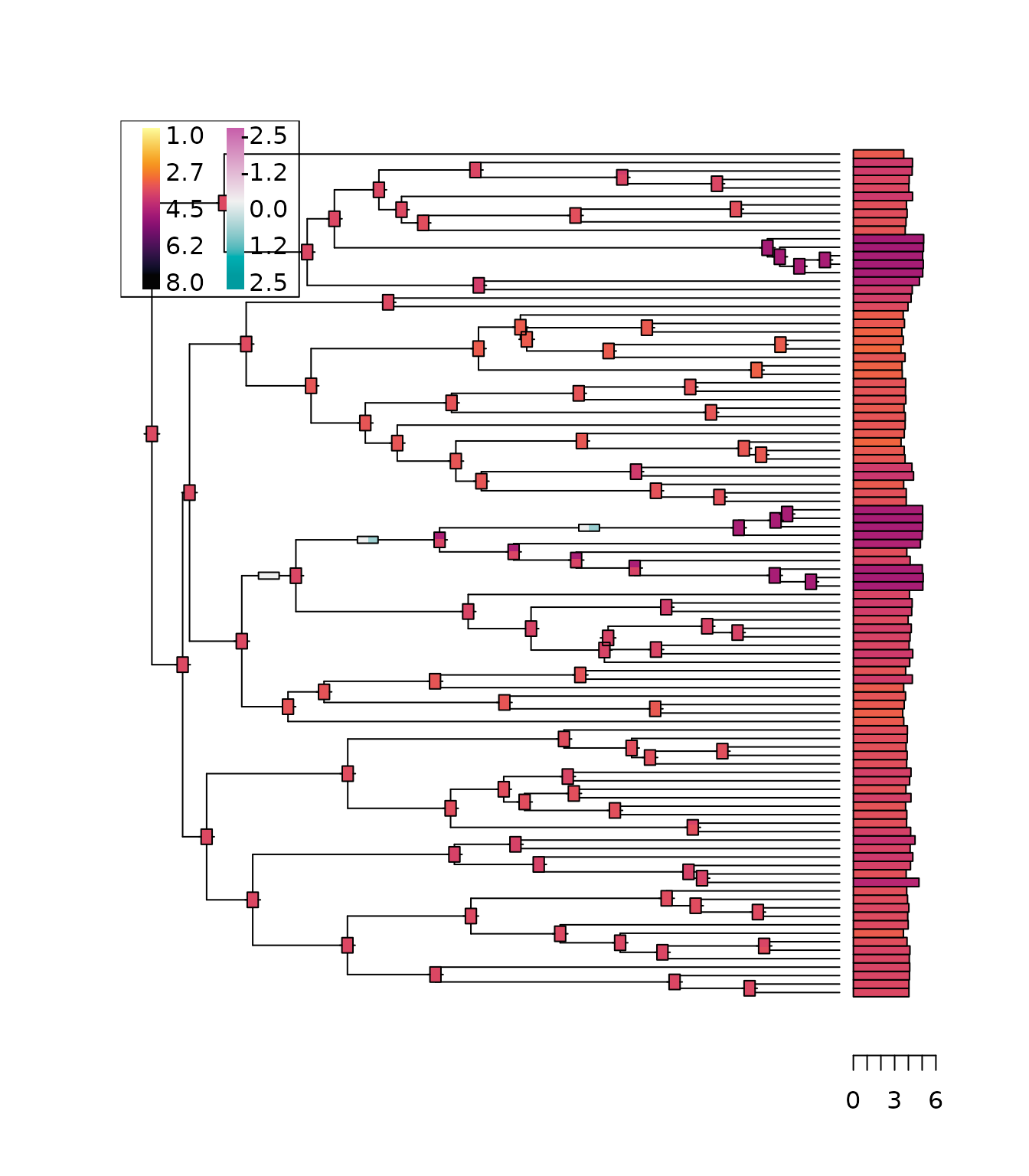
We can then plot schematics of these reconstructions on the tree, using thermo plots. To avoid any clutter, we only plot a few of them here.

plot_asr(cauchy_reml, anc = anc_reml, inc = inc_reml,
         show.tip.label = FALSE,
         width.node = 0.8, height.node = 1.8,
         width.edge = 1.5, height.edge = 0.8)

In this representation, trait or increment values are mapped to a common color scale. Each thermo plot represents the reconstructed node or branch posterior traits, with colors mapped to the modes of the distribution, and a width proportional to their relative weights. The function inherits from all the ape::plot function, and can be customized accordingly.

Mahler, D. Luke; Ingram, Travis; Revell, Liam J.; Losos, Jonathan B. (2013), Data from: Exceptional convergence on the macroevolutionary landscape in island lizard radiations, Dryad, Dataset, https://doi.org/10.5061/dryad.9g182 ↩︎

Paul Bastide