Plot Ancestral States Reconstructions

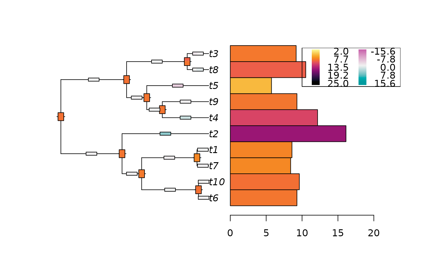
Plot the ancestral states reconstructions from a fitted Cauchy model.

plot_asr(
  x,
  anc = NULL,
  inc = NULL,
  common_colorscale = FALSE,
  x.legend = "topleft",
  y.legend = NULL,
  adj = c(0.5, 0.5),
  piecol = NULL,
  width.node = NULL,
  height.node = NULL,
  width.edge = NULL,
  height.edge = NULL,
  style = "bars",
  offset = 1,
  scaling = 1,
  x.lim = NULL,
  x.intersp = NULL,
  ...
)

Arguments

x

a cauphylm or fitCauchy object.

anc

(optional) an object of class ancestralCauchy, obtained with ancestral.

inc

(optional) an object of class ancestralCauchy, obtained with increment.

common_colorscale

If both plotted, should the ancestral states and the increment be represented by the same color scale ? Default to FALSE.

x.legend, y.legend

the x and y co-ordinates to be used to position the legend. They can be specified by keyword or in any way which is accepted by legend.

adj

one or two numeric values specifying the horizontal and vertical, respectively, justification of the text or symbols. By default, the text is centered horizontally and vertically. If a single value is given, this alters only the horizontal position of the text.

piecol

a list of colours (given as a character vector) to be used by thermo or pie; if left NULL, a series of colours given by the function rainbow is used.

width.node, height.node, width.edge, height.edge

parameters controlling the aspect of thermometers for the nodes and the edges; by default, their width and height are determined automatically.

style

a character string specifying the type of graphics; can be abbreviated (see details).

offset

offset of the tip labels (can be negative).

scaling

the scaling factor to apply to the data.

x.lim

a numeric vector of length one or two giving the limit(s) of the x-axis. If NULL, this is computed with respect to various parameters such as the string lengths of the labels and the branch lengths. If a single value is given, this is taken as the upper limit.

x.intersp

character interspacing factor for horizontal (x) spacing between symbol and legend text (see legend).

...

other parameters to be passed on to plot.phylo or phydataplot.

Value

None.

Details

The main plot is done with plot.phylo, the node annotation use nodelabels, and the tip data plot use phydataplot. Please refer to these functions for the details of the parameters.

The width of each color in the thermo plots approximately represents the weight of each node of the distribution, that is estimated by numerically integrating the density function around each mode. Function findpeaks is first used to find the modes and estimate their starting and ending points. Then function trapz estimates the integral of the density around the mode.

For an exact representation of a node posterior density, please plot it separately, using function plot.ancestralCauchy.

See also

cauphylm, fitCauchy, ancestral, increment, plot.phylo, phydataplot, nodelabels

Examples

set.seed(1289)
# Simulate tree and data
phy <- ape::rphylo(10, 0.1, 0)
dat <- rTraitCauchy(n = 1, phy = phy, model = "cauchy",
                    parameters = list(root.value = 10, disp = 0.1))
# Fit the data
fit <- fitCauchy(phy, dat, model = "cauchy", method = "reml")
# Reconstruct the ancestral states and increments
inc <- increment(fit, n_values = 100)
anc <- ancestral(fit, n_values = 100)
plot_asr(fit, inc = inc, anc = anc, offset = 3,
         width.node = 0.8, height.node = 0.5, 
         width.edge = 1.5, height.edge = 0.2,
         x.legend = "topright")