Posterior density of an increment

Compute the posterior density of a branch increment under a fitted Cauchy process on a phylogenetic tree.

increment(x, ...)

# S3 method for class 'cauphylm'
increment(x, node, values, n_values = 100, n_cores = 1, ...)

# S3 method for class 'cauphyfit'
increment(x, node, values, n_values = 100, n_cores = 1, ...)

Arguments

x: an object of class fitCauchy or cauphylm.
...: other arguments to be passed to the method.
node: vector of nodes ending the branches for which to compute the posterior density of the increment. If not specified, the reconstruction is done on all the possible edges.
values: the vector of values where the density should be computed. If not specified, the reconstruction is done for a grid of n_values values between -1.5 * maxdiff and 1.5 * maxdiff, where maxdiff is the difference between the larger and smaller tip value.
n_values: the number of point for the grid of values. Default to 100. Ignored if values is provided.
n_cores: number of cores for the parallelization. Default to 1.

Value

an object of S3 class ancestralCauchy, which is a matrix of posterior increment values, with nodes in rows and values in columns.

Details

This function assumes a Cauchy Process on the tree with fitted parameters (see fitCauchy), and computes the posterior ancestral density of trait increments at branches (ie, the difference between the traits value at the end and beginning of the branch), conditionally on the vector of tip values.

It computes the posterior density on all the points in values, that should be refined enough to get a good idea of the density curve.

Methods (by class)

increment(cauphylm): cauphylm object
increment(cauphyfit): fitCauchy object

References

Bastide, P. and Didier, G. 2023. The Cauchy Process on Phylogenies: a Tractable Model for Pulsed Evolution. Systematic Biology. doi:10.1093/sysbio/syad053.

Examples

set.seed(1289)
# Simulate tree and data
phy <- ape::rphylo(10, 0.1, 0)
dat <- rTraitCauchy(n = 1, phy = phy, model = "cauchy",
                    parameters = list(root.value = 10, disp = 0.1))
# Fit the data
fit <- fitCauchy(phy, dat, model = "cauchy", method = "reml")
# Reconstruct the ancestral increments
inc <- increment(fit)
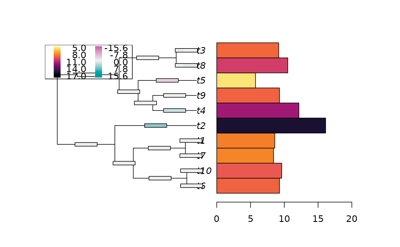
plot_asr(fit, inc = inc, offset = 3)

plot(inc, node = c(3, 8), type = "l")

# Refine grid for edges ending at tips 3 and 8
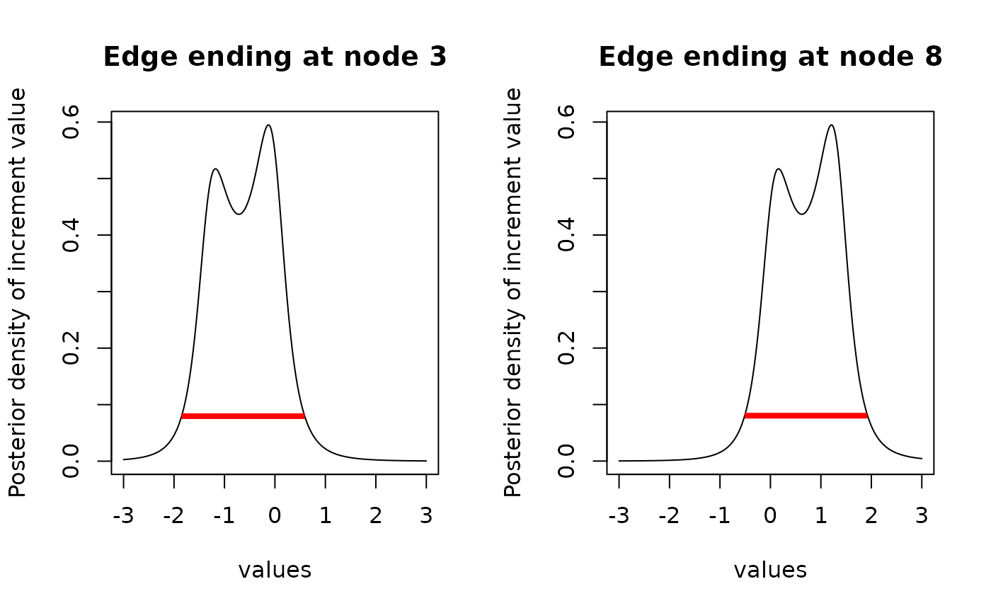
inc2 <- increment(fit, node = c(3, 8), values = seq(-3, 3, 0.01))
plot(inc2, type = "l")

# Find HDI
library(HDInterval)
hdi_inc <- hdi(inc2)
hdi_inc
#> $`3`
#>      begin  end
#> [1,] -1.85 0.59
#> attr(,"credMass")
#> [1] 0.95
#> attr(,"height")
#> [1] 0.07962038
#> 
#> $`8`
#>      begin  end
#> [1,] -0.51 1.92
#> attr(,"credMass")
#> [1] 0.95
#> attr(,"height")
#> [1] 0.0802933
#> 
plot(inc2, interval = hdi_inc, type = "l")